Function to Calculate Logistic Regression Over and Over Again
Logistic Regression Explained from Scratch (Visually, Mathematically and Programmatically)
Hands-on Vanilla Modelling Part III
A plethora of results appear on a minor google search "Logistic Regression". Sometimes it gets very confusing for beginners in information science, to get around the master idea behind logistic regression. And why wouldn't they be confused!!? Every different tutorial, article, or forum has a different narration on Logistic Regression (not including the legit verbose of textbooks considering that would kill the entire purpose of these "quick sources" of mastery). Some sources claim it a "Nomenclature algorithm" and some more sophisticated ones telephone call it a "Regressor", even so, the thought and utility remain unrevealed. Remember that Logistic regression is the basic building block of artificial neural networks and no/fallacious understanding of it could make it really hard to sympathize the advanced formalisms of data scientific discipline.
Here, I will endeavour to shed some low-cal on and within the Logistic Regression model and its formalisms in a very basic fashion in club to requite a sense of understanding to the readers (hopefully without confusing them). At present the simplicity offered here is at a cost of capering the in-depth details of some crucial aspects, and to get into the nitty-gritty of each aspect of Logistic regression would be like diving into the fractal (there will be no end to the give-and-take). However, for each such concept, I will provide eminent readings/sources that one should refer to.
For there are two major branches in the study of Logistic regression (i) Modelling and (ii) Mail service Modelling analysis (using the logistic regression results). While the latter is the measure of issue from the fitted coefficients, I believe that the black-box attribute of logistic regression has always been in its Modelling.
My aim here is to:
- To elaborate Logistic regression in the most layman way.
- To discuss the underlying mathematics of 2 popular optimizers that are employed in Logistic Regression (Gradient Descent and Newton Method).
- To create a logistic-regression module from scratch in R for each type of optimizer.
Ane last matter before nosotros go along, this unabridged commodity is designed by keeping the binary classification problem in mind in order to avoid complication.
ane. The Logistic Regression is NOT A CLASSIFIER
Aye, it is not. It is rather a regression model in the cadre of its heart. I will depict what and why logistic regression while preserving its resonance with a linear regression model. Assuming that my readers are somewhat aware of the basics of linear regression, it is easy to say that the linear regression predicts a "value" of the targeted variable through a linear combination of the given features, while on the other hand, a Logistic regression predicts "probability value" through a linear combination of the given features plugged inside a logistic office (aka inverse-logit ) given as eq(1):


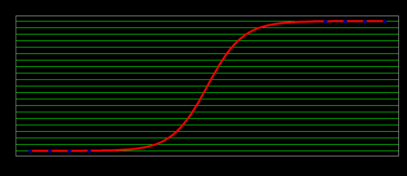
Hence the name logistic regression. This logistic function is a unproblematic strategy to map the linear combination "z", lying in the (-inf,inf) range to the probability interval of [0,1] (in the context of logistic regression, this z will be chosen the log(odd) or logit or log(p/1-p)) (run into the above plot). Consequently, Logistic regression is a type of regression where the range of mapping is confined to [0,1], unlike simple linear regression models where the domain and range could take any real value.

Consider unproblematic data with one variable and its respective binary class either 0 or 1. The scatter plot of this data looks something like (Fig A left). Nosotros come across that the data points are in the two extreme clusters. Practiced, now for our prediction modeling, a naive regression line in this scenario will give a nonsense fit (red line in Fig A correct) and what we really crave to fit is something similar a squiggly line (or a curvy "Southward" shaped blue rule in Fig A right) to explicate (or to correctly separate) a maximum number of data points.
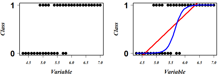
Logistic regression is a scheme to search this well-nigh optimum blue squiggly line. Now beginning permit's understand what each point on this squiggly line represents. given any variable value projected on this line, this squiggly line tells the probability of falling in Class i (say "p") for that projected variable value. So accordingly the line tells that all the bottom points that prevarication on this blue line have zero chances (p=0) of existence in course one and the top points that prevarication on it accept the probability of 1(p=one) for the aforementioned. At present, call up that I take mentioned that the logistic (aka changed-logit) is a strategy to map infinitely stretching space (-inf, inf) to a probability infinite of [0,ane], a logit role could transform the probability space of [0,1] to a space stretching to (-inf, inf) eq(two)&(Fig B).


Keeping this in heed, here comes the mantra of logistic regression modeling:
Logistic Regression starts with first Ⓐ transforming the space of course probability[ 0,i] vs variable {ℝ} (as in fig A right) to the space of Logit { ℝ } vs variable { ℝ } where a "regression like" fitting is performed by adjusting the coefficient and slope in order to maximize the Likelihood (a very fancy stuff that I will elaborated this office in coming section). Ⓑ Once tweaking and tuning are done, the Logit { ℝ } vs variable { ℝ } infinite is remapped to class probability[ 0,one] vs variable {ℝ} using changed-Logit (aka Logistic function). Performing this cycle iteratively ( Ⓐ →Ⓑ →Ⓐ ) would eventually effect in the virtually optimum squiggly line or the most discriminating rule.
WOW!!!
Well, you may (should) enquire (i) Why and how to do this transformation ??, (two) what the heck is Likelihood?? and (iii) How this scheme would lead to the most optimum squiggle?!!.
Then for (i), the idea to the transformation from a bars probability space [0,1] to an infinitely stretching real infinite (-inf, inf) is considering it will brand the plumbing equipment problem very close to solving a linear regression, for which we have a lot of optimizers and techniques to fit the most optimum line. The latter questions volition be answered eventually.
Now coming back to our search for the best classifying blueish squiggly line, the idea is to plot an initial linear regression line with the arbitrary coefficient on ⚠️logit vs variable space⚠️ coordinates first and then adjust the coefficients of this fit to maximize the likelihood (relax!! I volition explicate the "likelihood" when it is needed).
In our one variable case, we can write equation 3:
logit(p) = log(p/ane-p) = β₀+ β₁*v ……………………………….(eq 3)
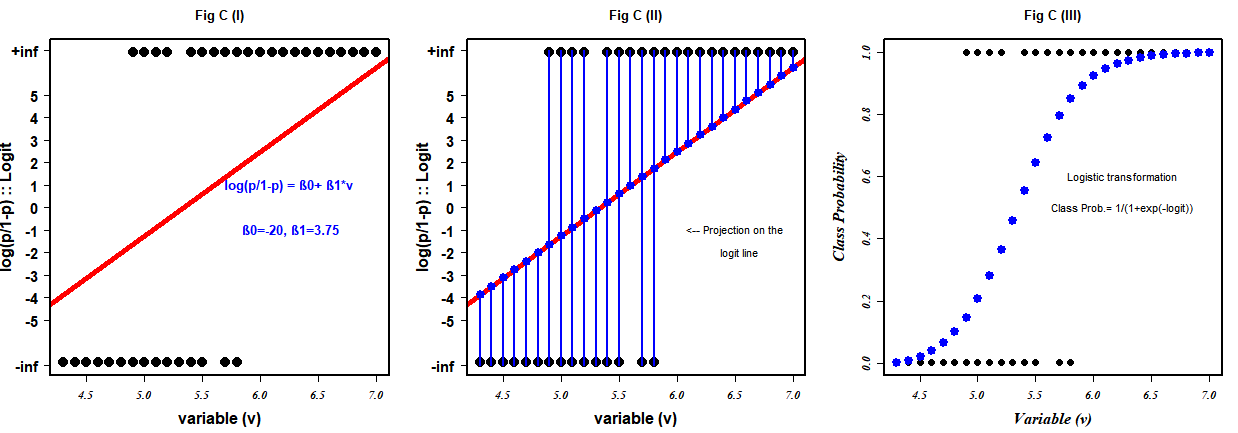
In Fig C (I), the red line is our arbitrary chosen regression line fitted for the data points, mapped in a different coordinate organization with β₀ (intercept) equally -20 and β₁(slope) equally 3.75.
⚠️ Notation that the coordinate space is not grade {0,1} vs variable {ℝ} simply its the Logit{ℝ} vs variable{ℝ}. Also, notice that the transformation from Fig A(right) to Fig C(I) has no effects on the positional preferences of the points i.e. the extremes as in equation 2 above, the logit(0)=-infinity, and logit(1)=+infinity.
At this point, let me reiterate our objective: Nosotros desire to fit the straight line for the information points in logit vs variable plot in such a way that it explains (correctly separates) the maximum number of information points when it gets converted to the blue squiggly line through inverse-logit (aka logistic role) eq(one). And so to achieve the best regression, a similar strategy of simple linear regression comes into play only despite minimizing the squared residue, the idea is to maximize the likelihood (relax!!). Since the points scattered on the infinity get in difficult to keep in an orthodox linear regression method, the trick is to project these points on the logit (the initial chosen/fitted line with the capricious coefficient) Fig C(Two). In this way, each data signal projected on the logit corresponds to a logit value. When these logit values are plugged into the logistic office eq(1), nosotros get their probability of falling in form 1 Fig C(III).
Annotation: This too can be proven mathematically likewise that: logit(p)=logistic⁻¹(p)
This probability can exist represented mathematically as equation four, which is very shut to a Bernoulli distribution, isn't it?.
P(Y = y|X = x) = σ(βᵀ x)ʸ · [1 − σ(βᵀx)]⁽¹⁻ʸ⁾ ; where y is either 0 or one..eq(four)
The equation reads that for a given data case x , the probability of the label Y existence y(where y is either 0 or ane) is equal to the logistic of logit when y=1 and is equal to (1-logistic of logit) if y=0. These new probability values are illustrated in our class {0,1} vs variable {ℝ} infinite equally blue dots in Fig C(III). This new probability value for a datapoint is what we call the LIKELIHOOD of that data signal. And then in uncomplicated terms, likelihood is the probability value of the datapoint where the probability value indicates that how LIKELY the point is to be falling in the class ane category. And the likelihood of the preparation label for the fitted weight vector β is nothing but the product of each of these newfound probability values equation v&six.
L(β) = ⁿ∏ᵢ₌₁ P(Y = y⁽ⁱ⁾ | X = x⁽ⁱ⁾ )………………….……….eq(5)
Substituting equation four in equation v we get,
L(β) = ⁿ∏ᵢ₌₁ σ(βᵀ x⁽ⁱ⁾)ʸ⁽ⁱ⁾ · [one − σ(βᵀx⁽ⁱ⁾)]⁽¹⁻ʸ⁽ⁱ⁾⁾ ………………eq(six)
The idea is to estimate the parameters (β) such that it maximizes the L(β). Even so, due to the mathematical convenience, nosotros maximize the log of L(β) and call its log-likelihood equation 7.
LL(β) = ⁿ∑ᵢ₌₁ y⁽ⁱ⁾log σ(βᵀ 10⁽ⁱ⁾) + (i− y⁽ⁱ⁾) log[1 − σ(βᵀ10⁽ⁱ⁾)]……..eq(7)
So at this point, I hope that our earlier stated objective is much understandable i.e. to discover the all-time fitting parameters β in logit vs variable space such that LL(β) in probability vs variable infinite is maximum. For this, there is no close form and so in the side by side department, I will impact upon two optimization methods (1) Gradient descent and (two) Newton'south method to find the optimum parameters.
2. Optimizers
Gradient Ascension
Our optimization first requires the fractional derivative of the log-likelihood function. So let me shamelessly share the snap from a very eminent lecture note that beautifully elucidate the steps to derive the partial derivative of LL(β). (Note: the calculations shown here use θ in identify of β to represent the parameters.)


To update the parameter, the steps toward the global maximum is:

so the algorithm is:
Initialize β and set likelihood=0
While likelihood≤max(likelihood){
Calculate logit( p ) = 10 βᵀ
Calculate P =logistic(Xβᵀ)= i/(1+exp(-Xβᵀ))
Calculate Likelihood L(β) = ⁿ∏ᵢ₌₁ ifelse ( y(i)=1, p(i), (1-p(i)))
Calculate first_derivative ∇LL(β) = Tenᵀ (Y-P)
Update: β(new) = β (old) + η ∇LL(β)
}
Newton Method
Newton's Method is another strong candidate among the all bachelor optimizers. Nosotros have learned Newton's Method as an algorithm to stepwise find the maximum/minimum point on the concave/convex functions in our early lessons:
xₙ₊₁=tenₙ + ∇f(xₙ). ∇∇f⁻¹(tenₙ)
In the context of our log-likelihood role, the ∇ f(xₙ) will exist replaced past the gradient of LL(β) (i.east ∇LL(β)) and the ∇∇f⁻¹(10ₙ) would be the Hessian H i.e. the second-order partial derivative of LL(β)). Well, I will caper the details here, but your curious brain should refer to this. Then, the ultimate expression to update the parameter, in this case, is given by:
βₙ₊₁=βₙ+ H⁻¹. ∇LL(β)
Here in the instance of logistic regression, the calculation of H is super piece of cake because:
H= ∇∇LL(β) = ∇ⁿ∑ᵢ₌₁[y − σ(βᵀx⁽ⁱ⁾)].ten⁽ⁱ⁾
= ∇ⁿ∑ᵢ₌₁[y − pᵢ].10⁽ⁱ⁾
= −ⁿ∑ᵢ₌₁ x⁽ⁱ⁾(∇pᵢ) = −ⁿ∑ᵢ₌₁ x⁽ⁱ⁾ pᵢ(1-pᵢ) (10⁽ⁱ⁾)ᵀ
thus, H= -XWXᵀ, where Westward=(P*(1-P))ᵀ I
So the algorithms are:
Initialize β and set likelihood=0
While likelihood≤max(likelihood){
Summate logit( p ) = x βᵀ
Calculate P =logistic(Xβᵀ)= 1/(one+exp(-Xβᵀ))
Calculate Likelihood Fifty(β) = ⁿ∏ᵢ₌₁ ifelse ( y(i)=ane, p(i), (i-p(i)))
Summate first_derivative ∇LL(β) = 10ᵀ (Y-P)
Calculate Second_derivative Hessian H = -Xᵀ (P*(1-P))ᵀI X
β(new) = β (old) + H⁻¹. ∇LL(β)
}
3. The Scratch Code
The data
The dataset that I am going to utilise for training and testing my binary classification model can be downloaded from here. Originally this dataset is an Algerian Forest Fires Dataset. Y'all can check out the details of the dataset here.
The Lawmaking
For the readers who hopped the entire article to a higher place to play effectually with code, I would recommend having a quick eyeballing through the second section as I take given a spet-wise algorithm for both the optimizer and my code will strictly follow that guild.
The training Role
setwd("C:/Users/Dell/Desktop")
set.seed(111) #to generate the same results as mine #-------------Preparation Function---------------------------------# logistic.train<- function(train_data, method, lr, verbose){b0<-rep(ane, nrow(train_data))
ten<-as.matrix(cbind(b0, train_data[,ane:(ncol(train_data)-ane)]))
y<- train_data[, ncol(train_data)]beta<- equally.matrix(rep(0.five,ncol(ten))); likelihood<-0; epoch<-0 #initiate
beta_all<-Zero
beta_at<-c(1,10,50,100,110,150,180,200,300,500,600,800,1000,
1500,2000,4000,5000,6000,10000) #checkpoints (the epochs at which I will record the betas)#-----------------------------Gradient Descent---------------------#
if(method=="Gradient"){
while( (likelihood < 0.95) & (epoch<=35000)){logit<-x%*%beta #Calculate logit(p) = xβᵀ
p <- one/( 1+ exp(-(logit))) #Summate P=logistic(Xβᵀ)= ane/(1+exp(-Xβᵀ))
# Likelihood: L(x|beta) = P(Y=1|10,beta)*P(Y=0|ten,beta)
likelihood<-1
for(i in 1:length(p)){
likelihood <- likelihood*(ifelse( y[i]==1, p[i], (1-p[i]))) #product of all the probability
}first_d<- t(10) %*% (y-p)#first derivative of the likelihood function
beta <- beta + lr*first_d #updating the parameters for a step toward maximization
#to run across inside the steps of learning (irrelevant to the chief working algo)
if(verbose==T){
ifelse(epoch%%200==0,
impress(paste0(epoch, "th Epoch",
"---------Likelihood=", round(likelihood,4),
"---------log-likelihood=", round(log(likelihood),4),
collapse = "")), NA)}if(epoch %in% beta_at){beta_all<-cbind(beta_all, beta)}
epoch<- epoch+ane
}
}#--------------Newton second society unequal method-------------#
else if(method=="Newton"){
while((likelihood < 0.95) & (epoch<=35000)){logit<-x%*%beta #Summate logit(p) = xβᵀ
p <- 1/( 1+ exp(-(logit))) #Calculate P=logistic(Xβᵀ)= 1/(1+exp(-Xβᵀ))# Likelihood: L(x|beta) = P(Y=1|10,beta)*P(Y=0|ten,beta)
likelihood<-ane
for(i in 1:length(p)){
likelihood <- likelihood*(ifelse( y[i]==1, p[i], (i-p[i])))
}first_d<- t(x) %*% (y-p)#first derivative of the likelihood role
w<-matrix(0, ncol= nrow(10), nrow = nrow(x)) #initializing p(ane-p) diagonal matrix
diag(w)<-p*(1-p)
hessian<- -t(ten) %*% due west %*% 10 #hessian matrixhessian<- diag(ncol(ten))-hessian #Levenberg-Marquardt method: Add a scaled identity matrix to avoid singularity issues
k<- solve(hessian) %*% (t(x) %*% (y-p)) #the gradient for newton method
beta <- beta + k #updating the parameters for a step toward maximization
if(verbose==T){
ifelse(epoch%%200==0,
print(paste0(epoch, "th Epoch",
"---------Likelihood=", round(likelihood,iv),
"---------log-likelihood=", round(log(likelihood),4),
collapse = "")), NA)}if(epoch %in% beta_at){beta_all<-cbind(beta_all, beta)} #just to inside the learning
epoch<- epoch+1
}
}else(break)
beta_all<-cbind(beta_all, beta)
colnames(beta_all)<-c(beta_at[1:(ncol(beta_all)-1)], epoch-1)mylist<-listing(as.matrix(beta), likelihood, beta_all)
names(mylist)<- c("Beta", "likelihood", "Beta_all")
return(mylist)
} # Fitting of logistic model
The Prediction Function
                logistic.pred<-role(model, test_data){                      test_new<- cbind( rep(1, nrow(test_data)), test_data[,-ncol(test_data)]) #adding ane to fit the intercept                                        beta<-equally.matrix(model$Beta) #excerpt the best suiting beta (the beta at final epoch)
                    beta_all<-model$Beta_all #extract all the betas at different checkpoints
                    ll<- model$likelihood #extract the highest likelihood obtained                                        log_odd<-cbind(as.matrix(test_new)) %*% beta #logit(p)                                        probability<- 1/(one+ exp(-log_odd)) # p=logistic(logit(p))
                    predicted_label<- ifelse(probability >= 0.5, 1, 0) #discrimination rule                                        k<-cbind(test_data[,ncol(test_data)], predicted_label) # actual label vs predicted label
                    colnames(k)<- c("Actual", "Predicted")
                    one thousand<- as.data.frame(thousand)                                        tp<-length(which(k$Bodily==1 & g$Predicted==1)) #true positive
                    tn<-length(which(m$Actual==0 & k$Predicted==0)) #true negative
                    fp<-length(which(m$Bodily==0 & grand$Predicted==i)) #false positive
                    fn<-length(which(k$Bodily==one & chiliad$Predicted==0)) #false negative                                        cf<-matrix(c(tp, fn, fp, tn), 2, ii, byrow = F) #confusion matrix
                    rownames(cf)<- c("i", "0")
                    colnames(cf)<- c("ane", "0")                                        p_list<-list(chiliad, cf, beta, ll, beta_all)
                    names(p_list)<- c("predticted", "defoliation matrix","beta", "liklihood", "Beta_all")
                    return(p_list)                                      } # to make prediction from the trained model
Data Parsing
                #importing information
data<-read.csv("fire.csv", header = T) #import
data$Classes<-every bit.numeric(ifelse(1:nrow(data)%in%grep("not",data$Classes), 0, 1)) # one hot encoding ; numeric conversion from label to ane or 0
information<-rbind(data[which(information$Classes==0),],
                  data[sample(size=length(which(data$Classes==0)),which(data$Classes==1)),]) #balancing the classes
data<-data[sample(i:nrow(data)),] #shuffling
data<-as.data.frame(data) #data to data frame
information<-lapply(data, every bit.numeric)
data<-as.data.frame(data)                #missing data handling
if(!is.null(is.na(data))){
                  data<-information[-unique(which(is.na(information), arr.ind = T)[,1]),]
}                #test train partition
partition<-sample(c(0,1), size=nrow(data), prob = c(0.viii,0.2), replace = T)
railroad train<-information[which(partitioning==0),]
test<-data[which(segmentation==1),]
Training → Testing → Results
                #-------------------------TRAINING---------------------------------#                mymodel_newton<- logistic.train(train, "Newton", 0.01, verbose=T) # Fitting the model using Newton method
mymodel_gradient<- logistic.train(train, "Slope", 0.01, verbose=T) # Fitting the model using Gradient method                #------------------------TESTING-------------------------------------#
myresult1<-logistic.pred( mymodel_newton, test_data = test) #prediction using Newton trained model
myresult2<-logistic.pred( mymodel_gradient, test_data = test) #prediction using Gradient trained model                #------------------------Results----------------------------------#
myresult1$`defoliation matrix`
myresult2$`confusion matrix`
The Results

The defoliation matrix obtained by both methods is the aforementioned. The accuracies obtained by both methods on the independent test set are 95.2% (quite good!!).

However, the best fitting coefficients β obtained by both methods are very dissimilar in terms of values. Newton'southward method took 3,566 epochs to obtain a likelihood of ane, while Slope descent took iii,539 to read the maximum likelihood of 0.999.
In terms of time taken, Newton's method took more time to attain the optimum in comparison to the gradient method because, in Newton'due south method, the solving inverse of Hessian makes it a fiddling computationally all-encompassing and fourth dimension-consuming algorithm.
Every bit y'all have noticed that I take captured the betas at various checkpoints during the training. This volition permit us to peep into the preparation process that is carried out while maximizing the likelihood (see ⇩⇩⇩⇩)


We can likewise peep into the fitting on the test set past the fully trained model


So at this indicate, I recollect I can reiterate to the reader that the primal nature of Logistic Regression is not of classification, rather it is of regression. Through substantiating a regression in its core performance, The Logistic regression gives output equally probability attached to a given instance. It is when a rule of >or≤ 0.5 or something is employed, the consignment of an instance to a particular discrete form is carried out.

Decision
If you are hither and so go get yourself a fine treat, yous are a real MVP. I promise my very casual elaboration on logistic regression gave y'all slightly better insights into the logistic regression. This article encompasses the concept, the underlying mathematics, and the programming of logistic regression. While the ideas here depict the bodily scheme, in that location are some out-of-scope aspects of the optimizers discussed here, in which the optimizing algorithm might fail to reach an optimum, more than details can exist found hither.
Feel gratis to download the entire code (Model and plots) from my git.
Source: https://towardsdatascience.com/logistic-regression-explained-from-scratch-visually-mathematically-and-programmatically-eb83520fdf9a
0 Response to "Function to Calculate Logistic Regression Over and Over Again"
Postar um comentário